Some of the familiar tasks while formulating coatings include finding a new solvent blend for a coating, ensuring the right level of “happiness” in all components of a coating, finding the best way to get adhesion to a substrate, and more.

These and others are solubility/compatibility issues. Thanks to Hansen Solubility Parameters (HSP), it is now possible to adopt a science-based approach for resolving solubility issues with speed and understanding. It’s a great opportunity to avoid hours of unfocused trials. 

Better Coatings via Science-Based Formulation Using HSP

So you need to find a new solvent blend, or you need to incorporate a new polymer, or someone has offered a new pigment or nanoparticle that promises improved properties. How do you use the minimum effort to get the maximum balance of desired properties? 

Clearly, it is important to understand the different solubility and compatibility issues between your components. You can try to do this via vague words like hydrophobic/hydrophilic or polar/non-polar, but these are too vague to be of much use. We need numbers to formulate scientifically, and in particular, we need a good measure of how “like” or “unlike” any two molecules might be. To get a measure of likeness, we must start with three numbers that describe each chemical, polymer, particle or additive used in our coating formulation. 

Why three? Because two is too small and four is too complicated. Though, there is always an implicit fourth parameter, the molecular size, which is not discussed further in this article. This article describes:

• What those three numbers are;
• How you can determine them;
• How you can use them in three specific areas of coatings: coating a polymer, ensuring compatibility between the ingredients in the coating, and ensuring compatibility between coating and substrate so it sticks well.      

What Are the Three Hansen Solubility Parameters?

The three parameters capture the essence of three familiar features of any molecule: 

• Dispersive aspect (dD);
• Polar aspect (dP);
• Hydrogen-bonding aspect (dH).

Coatings formulators can readily appreciate the polar and hydrogen-bonding aspects. The dispersive part is less used, but is still intuitive. All molecules are held together via van der Waals or dispersive forces, and these forces differ for different molecules. Aromatics, for example, have a broad electron cloud, so they self-interact more strongly than the alkanes, which have a tight cloud. Many formulators, including myself, have gone wrong by not recognizing the importance of this apparently boring parameter.

The three numbers, dD, dP and dH, are the Hansen Solubility Parameters, and by looking at the list of some common solvents, you will see that the HSP values are not at all mysterious, and agree with intuition and common sense (Table 1). 

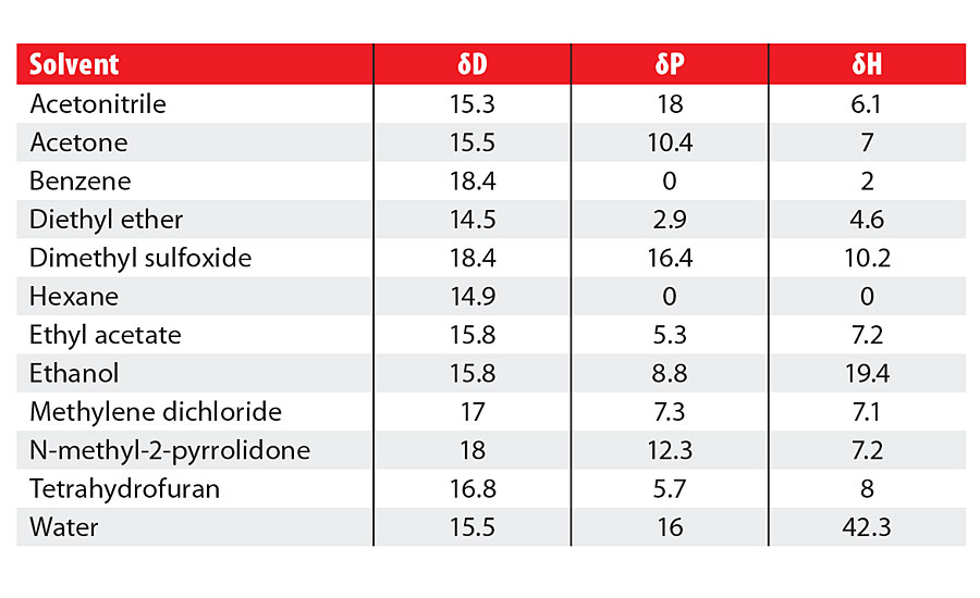
Acetonitrile, for example, has a high dP value because the -CN group provides a high dipole moment. But although it can form weak hydrogen bonds, their weakness means that its dH value is not very large.

Ethanol is fairly polar with a significant dP value but, as we would expect from such a strong hydrogen-bonded solvent, it has a much larger dH value.

Acetonitrile and ethanol have relatively small dD values, whereas benzene and DMSO both have higher dD values because they have large electron clouds around them. Benzene’s dD makes up most of its HSP, whereas DMSO is a rather special solvent with high values for all three parameters.

Hexane is a low dD solvent with no dP or dH, while acetone and ethyl acetate have middle-of-the-road values.

Measuring How “Like” Two Molecules Are

Given that we have the HSP values, we are set to find how “like” or “unlike” two molecules are. This is calculated as the “distance”, D, in 3D space between any pair, via the famous HSP formula for 3D distance, which, for various reasons, privileges dD by a factor of 4:

D² = 4(dD1-dD2)²+(dP1-dP2)²+(dH1-dH2)². If D between molecules is less than, say, 4 then they are a reasonable match. When D is greater than, say, 8 the molecules are a poor match.

Intermediate values are a matter of judgment. We can use these D calculations to make a rational choice. Suppose you have a target molecule and a list of molecules that, for other reasons, you are thinking might be useful. You calculate the D value between the target and each of the molecules and then sort them from high (bad) to low (good).

You can then ignore all the high-D molecules and form the low-D molecule, which meets your other requirements, such as cost or volatility. Typical examples for such a process would be if the target is a polymer and the molecules are solvents. Equally, HSP works very well when the target is a pigment or nanoparticle and the aim is to create a coating or a stable polymer blend.

What if no molecule matches all your coatings formulation requirements? If there was a single molecule that met all your requirements, that would be ideal. But, in reality, this is rarely the case. Happily, you can create a rational blend of two molecules, each of which has a high D value and is unsuitable on its own, but that you would like to use for other reasons. 

Suppose that each molecule has a reasonable match of dD with your target, but one has a high dP and low dH, and the other has a low dP and high dH. The HSP of a blend is simply the weighted average of the components. So, in this case, the dP and dH of the blend can be tuned to be a close match to your target. 

Therefore, a blend of molecules, each of which is unusable because of a high D that becomes usable, can work. Hansen worked out this blending trick and it has been one of the main reasons for the success of HSP. 

So now all you need are the HSP values so you can do the calculations. Where can you find them?

Finding the HSP Values

The good news is that for all the common solvents, the newer green solvents and for many polymers and additives, the HSP values are known and in the public domain. HSP data for thousands of coatings ingredients is available on SpecialChem along with the list of compatible products, thanks to contributions by the members of the Science-based Formulation Group, SBFG.* What about your own special chemical, polymer or additives? How do you determine the HSP of your own resin, particle or additive? The answer is that HSP values can be measured via two techniques (Figure 1). You can do this in-house or contract it out to those who offer it as a commercial service. 

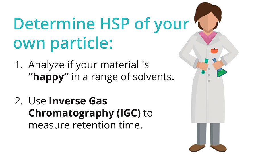
The first technique is based on your judgments about whether your material is “happy” (soluble, swellable, dispersible, etc.) or “unhappy” in a set of solvents that you have chosen because they span HSP space. The set of “good” solvents defines a sphere, the center of which gives the HSP with a radius that defines the range of solvents that would be compatible.

The second technique uses Inverse Gas Chromatography (IGC), which uses your sample as the stationary phase and measures how strongly each of a set of probe molecules interacts – as judged by retention time. The standard technique is more widely used. The IGC technique is especially useful for oligomers, surfactants and dispersants, and other molecules that are so fluid at room temperature that the standard test gives too many “good” solvents and too few “bad” ones.

Finding the Right Solvent (Blend)

Principle: Given a known HSP for a polymer or pigment you wish to coat, it is very easy to find an effective solvent for the material; get a list of solvent HSP values, calculate the distance from the material and choose the solvent with the shortest distance. But real life is not like that! 

We don’t want just an effective solvent, we want a usable solvent. So cost, odor, VOC level, hazard rating, etc. all become significant factors in our choice. Almost always, the best solvent in terms of HSP is unsatisfactory for other reasons, and as we go down our list in terms of increasing distance, we might fail to find a satisfactory compromise. This is when the power of HSP is fully revealed. 

Making a “Perfect Solvent” Out of Two “Bad Solvents”

Imagine that our solute has an HSP represented by the green dot inside the green sphere in Figure 2, and that we have two bad solvents which, by definition, are outside the sphere.

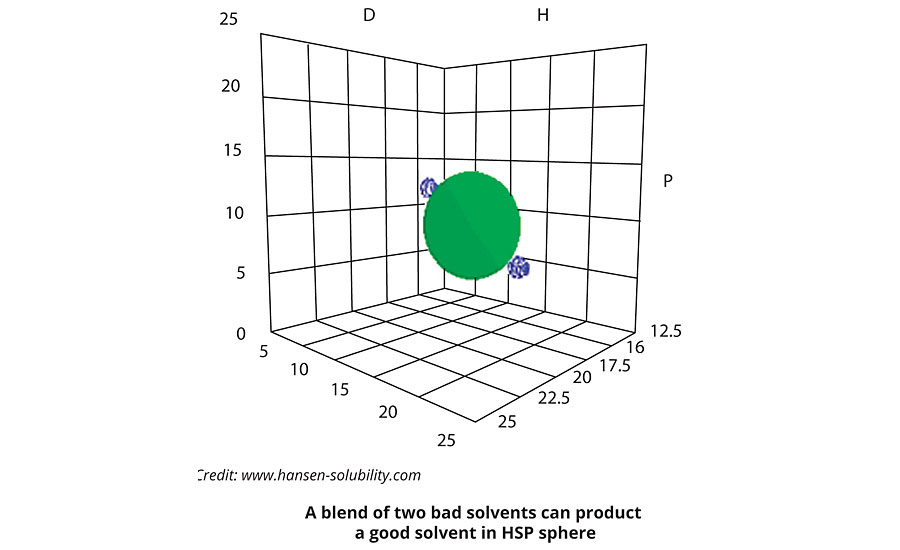
In the figure, those bad solvents happen to be exactly opposite to each other. Now make a blend of 50:50. The HSP of a blend is the volume weighted average of the two components which, in this case, would make this blend a perfect solvent for the solute. If you try this in practice, you find that you really can make a good solvent from two bad solvents, or take two OK solvents and create a really good blend. 

All it needs is the HSP of your target. An optimum blend can readily be found with a list of suitable solvents via human judgment or a computer algorithm with weightings for factors such as cost, greenness, etc.

Fine-Tuning the Evaporation Rate

If we know the relative evaporation rates of the individual solvents and their individual distances; we can even tune what happens to a coating during evaporation. When the solution is relatively dilute we can get a cheap, but not very good solvent. As the coating dries, we often want the polymer to stay in solution for as long as possible to be relaxed and glossy. This means that the less volatile solvent should be a closer match.

Figure 3 shows an example where the distance (called Ra) goes from 5.2 at the start (not great, but ok) to 3 as the ethyl acetate evaporates faster than the cyclohexanone.

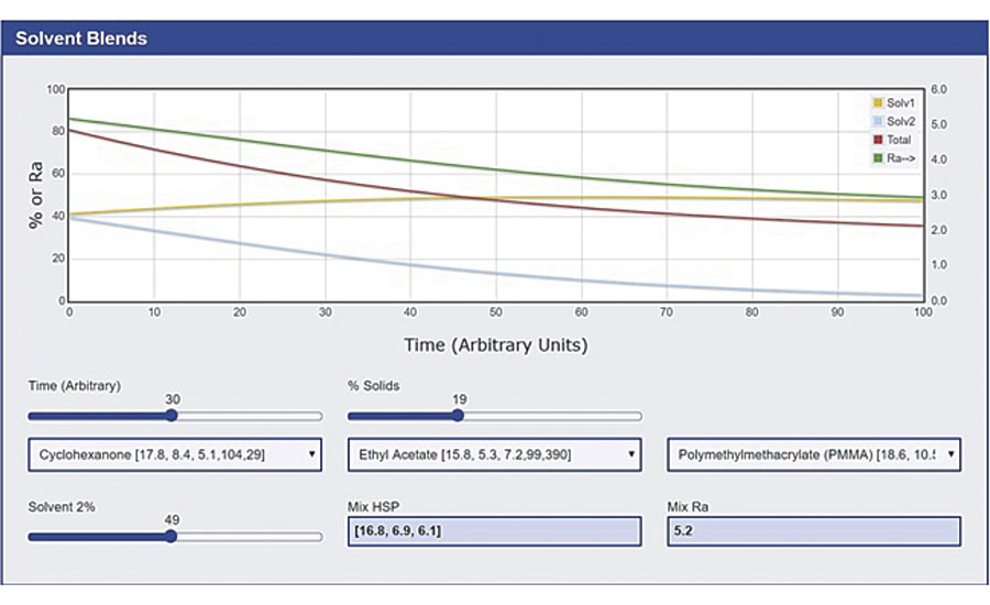
HSP Distance Transition in Solvent Blends

If you want the coating (or a component in it) to crash out quickly, you tune the blend so that the better solvent is more volatile.

Producing a Rational Blend of “Greener” Solvents

One area where solvent blends are especially important is in the replacement of a toxic or environmentally unfriendly solvent with a greener alternative. Using your current solvent as the target, you can take any convenient list of green solvents and find the closest match. 

It is usually the case that no single solvent is good enough, so you have to produce a rational blend of the greener solvents. This HSP method for creating greener blends has been proven to work many times – in the lab and in the real world of cleaning. For example, creating safer solvents for cleaning up after a printing or coating run. Once, some of my operators complained about one cleaning solvent blend, and they asked me to use it myself. It was terrible in two senses: it was smelly and unhealthy, and it was so volatile that the polymer would re-deposit before it had been properly removed.

Using HSP and being limited to the nicer solvents we happened to have in-house, I quickly created a pleasant, low-odor, low-volatile blend. When we tried it, it was useless if the previous cleaning regime was followed. But, by putting it onto the equipment as soon as it needed cleaning, attending to other jobs and returning, we found that the solvent blend was still, and had time to dissolve the polymer. A simple wipe removed most of the polymer, and a quick clean with the old blend finished the process. Far less work for far better results – and much safer. 

Polymer Compatibility with Other Ingredients

Polymer-Polymer Compatibility

From the formal theory behind HSP, it is possible to prove a rather shocking fact that has been validated experimentally. That is, most polymers are insoluble in most other polymers. For instance, PMMA is not soluble in PEMA. It turns out that for mutual compatibility, the HSP distance between two polymers has to be less than 0.1, which is impossible.

Our real-world experience is that there are plenty of reasonable polymer blends between related polymers. Here we have a difference between “reasonable” and “thermodynamics”. 

Moderate-molecular-weight PMMA and PEMA are easily mixed together, and under normal circumstances will not phase separate. The thermodynamic limit applies to high molecular weights and long times at high temperatures, allowing the polymers to reach equilibrium. So if you want practical polymer blending with a low risk of long-term phase separation, a low HSP distance is a good starting point. 

If you use a more elaborate version of HSP, which splits dH into donor/acceptor, you can find that polymers with relatively large distances, such as polyvinyl phenol and polyvinyl acetate, can form stable blends via donor/acceptor interactions.

Polymer-Other Additive Compatibility

When it comes to other additives in coatings, such as pigments, nanoclays, etc., low HSP distance is the first criterion for long-term stability. By knowing the HSP of your additives from your suppliers or by measuring the values for your own special ingredients, it becomes much easier to create “happy” formulations where everything likes to be with everything else.

Many long-term problems with coatings are caused by incompatibilities that could easily have been identified early on via HSP distance. For those who coat onto polymers that contain plasticizers, having a good knowledge of their HSP values makes it easier to control whether the plasticizer accumulates at the interface (which can be dangerous) or is absorbed relatively easily into the coating.

Coating and Substrate Adhesion

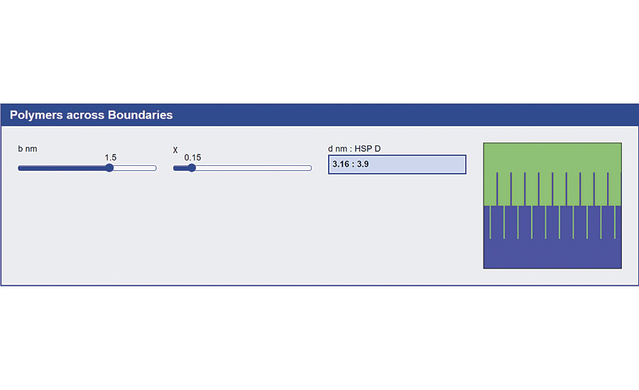
The best way to get adhesion across a polymer-polymer interface (i.e. the polymer in your coating adhering to the polymer of the substrate) is to have polymer chains crossing from both sides and becoming entangled. How can we calculate the chances of two polymers being able to intermingle and entangle to the required amount? A rather simple formula from Helfand relates the intermingling distance to the c parameter and, therefore, to HSP distance (Figure 4). 

Because the mythology that adhesion depends on surface energies is so widespread (even though surface energies are 1,000 times too small to be relevant) this powerful way to understand adhesion across interfaces is far too little known. But those who know it can attest to its power in being able to formulate correctly.

And it’s not just polymer-polymer. We often have a non-polymer surface and need to attach a primer molecule to aid adhesion. The primer needs to be long enough to tangle and compatible enough to be happy to associate with the polymer. So, finding the HSP of the primer is vital for success.

But however much the Helfand formula tells us we might get intermingling, the polymers are not going to cross the interface unaided. For heat sealing, we have temperature and time. For coating, we have solvents.

If one polymer is being delivered from the solvent then, of course, there must be good polymer-solvent compatibility, as discussed earlier. But we also need the solvent to attack the polymer onto which we are coating. Attack, yes, but not too much or we destroy the surface. 

Tuning the solvent to have enough “bite” into the surface to enable entanglement to take place (i.e. over a few nm) without destroying the surface (defects on the µm) scale is another job for HSP. 

Conclusion

For more than 50 years, HSP values have proven themselves in the world of formulations. Common tasks such as finding good solvents (or blends) or ensuring compatibility between components in a formulation become much more rational and efficient when the HSP values of all the key ingredients are known, either from your suppliers or internally, and HSP distance calculations are used routinely to find the best combinations

For more information, visit www.specialchem.com/