Degree of particle dispersion in a liquid paint or dry paint film affects practically every important property of these systems, including viscosity, touch-up, rub-up, scrub resistance, porosity, gloss, appearance of defects, and, for opacifying particles like TiO2, hiding power and tinting strength. Numerous methods have been devised to quantify degree of dispersion, but most are comparative rather than absolute, especially those that pertain to dispersion in the dry film (e.g., comparing hiding power to a standard). We detail a technique, based on electron microscopy and image analysis, of quantifying degree of TiO2 dispersion in a paint film. Results clearly indicate flocculation in some paints and, more importantly, put an upper limit on the potential for improvement of pigment dispersion.

Background

Pigmentary titanium dioxide is found in virtually all modern coatings, except those that are clear or extremely dark, because of its high opacity. Efficient use of TiO2 requires the particles be well dispersed in the final paint film, since close particle-particle interactions decrease the scattering efficiency of TiO2 and, thereby, its opacity.1-3 Good dispersion can be a challenge, however, because small particles tend to agglomerate (flocculate) due to Van der Waals attractions.4 Without some intervention from the coatings producer, the particles in a paint film would be significantly more poorly distributed than a random distribution. By attaching charged dispersant molecules to the pigment surface, however, the coatings manufacturer can improve overall dispersion. Perfect dispersion would require all particles to be evenly spaced from one another, but a more practical goal would be for the particles to be better dispersed than a random distribution (i.e., for electrostatic repulsions to completely overcome Van der Waals attractions).

Measuring the degree of particle dispersion in a paint film is problematic. Since poor dispersion results in poor hiding and low tint strength, these two measurements are often used as a proxy for degree of dispersion. This approach has the advantages that (a) it directly measures the attribute of interest (coatings users are interested in hiding power, not particle distribution per se), and (b) it is relatively easy to do. In addition, correlations can be drawn between dispersion parameters (energy, ingredients, equipment, etc.) and degree of dispersion, and empirical relationships developed that allow for performance optimization and for the development of theories explaining dispersion behavior. However, poor dispersion is possible by a number of mechanisms (poor initial dispersion, flocculation on drying, crowding due to other solid particles, etc.), and a detailed understanding of the state of dispersion is not possible through hiding power measurements alone. Instead, microscopic examination of the paint film is required.

Although microscopic examinations lend themselves well to comparative studies and to qualitative conclusions, a quantitative understanding of the degree of dispersion cannot be made through simple visual observations of electron micrographs. This is partly due to the human tendency to see patterns where none exist - whether it is mythological figures in the stars or meaningful images in the Rorschach ink-blot test - and our inability to intuitively judge, except in extreme cases, whether a distribution of objects is truly random, is somewhat ordered, or is artificially disordered (agglomerated).

In this paper we detail our efforts to quantitatively characterize TiO2 pigment dispersion in paint films. Our goal is to develop computer algorithms to analyze paint film images and quantify dispersion. To do this, we have developed a three-step procedure:

1. Collection of an image of the paint film that is suitable for particle coordinate determination;

2. Determination of coordinates for each particle center; and

3. Analysis of the coordinates in a way that meaningfully characterizes the degree of pigment dispersion, and that allows comparison between different images and to an idealized random distribution of particles.

Technical Approach - Imaging and Determination of Particle Coordinates

There are few constraints on the type of paints examined except that they must be relatively homogenous, since any gross differences in dispersion from one region of the film to another imply a different sort of issue than is under consideration in this paper. Related to this, the areas of the images to be analyzed must be large enough to be representative of the film, yet small enough to be manageable. As a rough guide to image size, we note that the precision of any image analysis is ultimately limited by counting statistics, and this limit is inversely proportional to the square root of the number of particles.5 Therefore, the best measure of image size is not the area of the image, but the number of particles within the image. In our work we have found images with between 500 and 1,000 particles to be tractable and to yield meaningful results.

Paints of interest were produced by standard procedures and drawn down on black Mylar® or the standard black and white cards routinely used for hiding power measurements. Once dried, 3-mm disks were punched and carbon coated for SEM analysis.

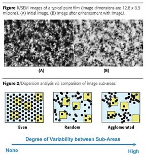
SEM images were taken using a Hitachi S-5000SP operated at 10 KV and typically at a magnification of 10,000x. Under these conditions, the pigment particles closest to the film surface can be discerned as white blurs, but the quality of these images is generally too poor to resolve all particles satisfactorily (Figure 1A). Images were therefore enhanced using ImageJ software.6 Images were first inverted (i.e., the negative was made), then smoothed using three passes through a median filter, ultimately giving an image similar to those seen using backscattering SEM (Figure 1B).

The coordinates of the particle centers can be determined with ImageJ either automatically or manually. In our experience, manual determination is preferred, as the automatic procedure incorrectly interprets groups of particles that are close to, or in contact with, one another as single, large particles. Note that these close interactions are precisely what is of interest to us, since they are responsible for hiding power losses, and so the errors introduced through automatic determination have a direct and negative impact on the results of subsequent data analysis.

Technical Approach - Analysis

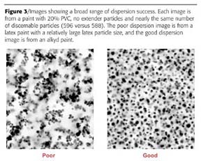
With the coordinates of particle centers in hand, the next step is to develop computational algorithms that can meaningfully quantify dispersion. This step is deceptively difficult - it is relatively easy to recognize and qualitatively characterize the dispersion quality of images, but quite difficult to derive quantitative data from these qualitative characterizations. For example, the three images in Figure 2 of black particles dispersed through blue fields can be described as differing in amount of "order", degree of "clumpiness", or level of "uniformity"; but how does one translate these descriptions into an algorithm amenable to encoding into a computer program?

One way of overcoming this difficulty is to recognize that these qualitative descriptions apply to each image taken in its entirety, but we do not need to limit our thinking to this. We have had success by taking a different approach to characterizing the differences between the images. We divide the images into smaller sub-areas (shown in yellow in Figure 2), measure some aspect of dispersion within each sub-area, and then compare these values to those for other sub-areas of the image. In a highly ordered system, every sub-area looks essentially the same, and there is very little variability when comparing sub-areas. In highly agglomerated systems, the opposite is true - a significantly higher degree of variability is seen between the sub-areas than would be expected for a random distribution of particles.

There are two key elements to this approach: how the images are divided into sub-areas and how the particle arrangement in each sub-area is measured. Rather than choose a single method for each of these key elements, we have found it more informative to choose two methods for each, thus giving us a total of four techniques for quantifying dispersion.

In the first method of dividing the image into sub-areas, the entire image is systematically probed: a 100 x 100 array of points is conceptually overlaid on the image, and the environment around each of these points is characterized by the two methods described below. A total of 10,000 points, which we will refer to as "array points", are probed in each image. The second method of dividing the image into sub-areas is to consider only the TiO2 particles: the immediate environment around each particle is characterized by the two methods detailed below.

For both methods of dividing the images into sub-areas, the area around each probe point is characterized the same way; the methods of dividing the image differ in how the probe points are chosen (either systematically across the entire image, or centered on each pigment particle). The benefit of the first method is that information is obtained uniformly from the entire image (even those regions that have few TiO2 particles), while the benefit of the second method is that it focuses on TiO2 particles and the interactions between them - that is, precisely the interactions that influence the optical efficiency of the pigment particles.

Once the probe points are chosen, the immediate environment around each is characterized by one of two methods. The first is to simply count the number of pigment particles within a given distance around the probe point. We have found it convenient to choose a distance such that, on average, 10 particles are expected to be found, rather than to arbitrarily choose a specific distance, because in this way the results for paints made at different PVC values can be directly compared. With this method the histogram of results expected for a truly random distribution of particles is simply the Poisson distribution for an average count of 10.

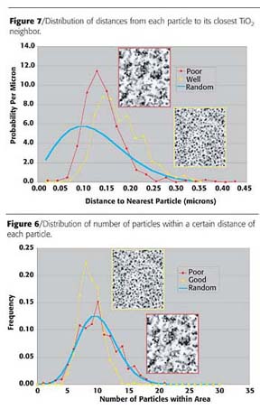
Alternatively, we can characterize dispersion in the local area of the probe points by determining the distance from the probe point to the closest pigment particle. The distribution of these distances is dependent on the degree of TiO2 pigment dispersion - for example, if the dispersion were completely uniform, then each probe point would be a short distance from a pigment particle, whereas if the dispersion were very poor (i.e., if there is a high degree of agglomeration), then some probe points would be very far from a pigment particle, since there will be large areas that are nearly free of particles. In addition to determining the distribution of closest particle distances for a given image, a theoretical distribution can be calculated for these distances assuming a truly random sample by applying Poisson statistics.

Example Application

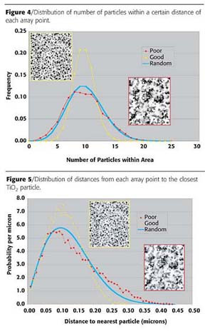
The four techniques for quantifying pigment dispersion were used to characterize the images shown in Figure 3. These images represent extremes in the range of degree of dispersion that we have observed for a large number of different paint systems. For each of the four quantification techniques, the results for the two images are compared to each other and to the result expected for a random distribution of particles (Figures 4 through 7).

Figure 4 shows the distributions of number of particles within a certain distance of each of the 10,000 array points probed on each image, and compares these distributions to that calculated for a truly random arrangement of particles. There are several noteworthy aspects of these three curves. First, it is clear that the distribution curves for the well-dispersed image and the poorly dispersed image are different from one another and are different from the curve calculated for a random distribution. Importantly, the measured curves differ from the random curve in opposite ways - every time the curve for the good-distribution image is above the random curve, the curve for the poor-dispersion image is below it, and vice versa. This indicates that the particles in one image are better dispersed than random and those in the other image are worse dispersed than random (i.e., are agglomerated). The good dispersion curve differs from the random curve in that it is sharper - that is, the environments of the array points are more similar to one another than would be the case if the particles were randomly dispersed - while the poor dispersion curve differs from the random curve in that it is broader, implying that the variability between the different array points is greater than can be explained by chance. Finally, note that the deviation from random is less pronounced for the poor dispersion image than for the good dispersion image - that is, the distribution of particles in the poor dispersion image is only very slightly worse than random, whereas the distribution of particles in the good dispersion image is significantly better than random.

Figure 5 shows the distances of each of the 10,000 array points probed in each image to the nearest pigment particle. Again the distributions of distances from the two images differ from the calculated distribution for a random arrangement of particles, and again they differ in opposite ways. The distribution of distances is sharper for the good dispersion image, consistent with the fact that there is less variability between different sub-areas in this image than there is between different sub-areas of the poor dispersion image. As in Figure 4, the curve for the poor dispersion image is closer to random than is the curve for the good dispersion image.

Figure 6 shows the number of neighboring particles within a certain distance from each pigment particle. These curves have the same general features as those in Figure 4, except that there is more noise in them. This is because there are far fewer data points in these curves compared to those in Figure 4. In Figures 4 and 5 a total of 10,000 points were probed (from a 100 x 100 array). In Figures 6 and 7 slightly fewer than 600 data points were probed (one data point for each pigment particle). That said, the major conclusion regarding Figures 4 and 6 is the same - the distributions of number of close particles in the two images are significantly different from one another. In this case, the good dispersion image differs substantially from random, but the poor dispersion picture cannot be distinguished from random, in part because of the higher level of noise in the data.

Finally, Figure 7 shows the distributions of distances from each particle to its nearest neighbor. Again there is a significant deviation of both curves from the theoretical curve for random, but in this case the curves differ in a similar way. For both images there are essentially no contacts below about 0.1 microns, and there are a large number of contacts between 0.1 and 0.2 micron. The lack of contacts at very short distances (< 0.1 micron) reflects the fact that it is the distances between particle centers that are measured, and there is a non-zero lower limit on these distances because when particles touch, their centers remain separated. Center-to-center contacts of between 0.1 and 0.2 microns represent particles that are touching one another; as expected, there are far more of these intimate contacts in the poor dispersion image than in the good dispersion image. Indeed, nearly all the particles are in contact with at least one other particle in the poor dispersion image, as evidenced by the fact that there are very few closest neighbor distances greater than 0.2 microns in this image.

Conclusions

A technique has been developed to quantify the degree of pigment dispersion in a paint film. Using this tool, a paint formulator can compare on an absolute basis the degree of dispersion of one paint film to another, even for films with different PVCs or resins, and can compare degree of dispersion to that expected for a random distribution of pigment particles. This information can guide the formulator to the conditions necessary for optimal dispersion, can offer evidence for different theories regarding dispersion, and can provide a useful indication of how close (or far) from ideal dispersion a given paint is (i.e., whether further formulation work would yield improved dispersion).

The technique consists of imaging the paint films with an electron microscope, determining the coordinates of the particle centers and analyzing these coordinates using four algorithms that divide the image into a large number of sub-areas, then comparing the particle attributes in each sub-area with those in the other sub-areas. A high degree of variability between sub-areas is indicative of poor dispersion, whereas a low degree of variability between sub-areas implies that the pigment particles are in identical environments, which is only possible when the particles are well dispersed.

References

1 Fields, D. P.; Buchacek, R.J.; Dickinson, J.G. Maximum TiO2 Hiding Power - The Challenge. J. Oil Colour Chem. Assoc. 1993, 2, 87.
2 McNeil, L. E.; French, R.H. Multiple Scattering from Rutile TiO2 Particles. Acta Materialia 2000, 48, 4571.
3 Thiele, E.S.; French, R.H. Light-scattering Properties of Representative, Morphological Rutile Titania Particles Studied Using a Finite-Element Method. J. Am. Ceram. Soc. 1998, 81, 469.
4 Everett, D. H. Basic Principles of Colloid Science; Royal Society of Chemistry Paperbacks, 1988.
5 Box, G.E.P.; Hunter, W.G.; Hunter, J.S. Statistics for Experimenters: An Introduction to Design, Data Analysis, and Model Building; John Wily & Sons, Inc., 1978.
6 ImageJ is a free public domain image analysis program available from the U. S. National Institute of Health website (http://rsb.info.nih.gov/ij/).

This paper was presented at the 8th Nürnberg Congress, Creative Advances in Coatings Technology, April 2005 in Nürnberg, Germany. The Congress is sponsored by FPL, PRA and the Vincentz Network.