Editor's Note: This article is Part 13 in a series; see PCI, September 2005, for the previous installment.

Predictive Equations

In a previous article, we discussed how to select experiments for factorial designs.1 Factorial designs are best used when studying categorical and continuous variables. Categorical variables include non-numeric variables, like lots of raw materials, equipment, methods and personnel. Categorical factorial designs are even used in the social sciences to differentiate between different modes of education or psychiatric treatment. A factorial design can tell if units within a category are statistically different. Continuous variables are numeric variables, like time, temperature, speed and pressure. Factorial designs on continuous variables can be used to draw response surfaces and quantify experimental variation. They are used to optimize manufacturing procedures and stabilize test methods.

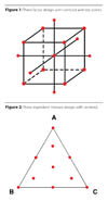
A graphical depiction of the factorial design experiments that would allow the calculation of a quadratic predictive equation for three variables is given in Figure 1.

The results of a factorial design on continuous variables can be quantified in a predictive equation. As an example, property as a function of two, X, process variables, is given in Equation 1.

Property (X) = a0 + a1X1 + a2X2 + a12X1X2 + a11X12 + a22X22 (1)

The performance property could be a factor like product yield, viscosity, hardness, gloss retention, etc. Any continuous variable and even some ranking2 variables can be the performance property.

Similarly in the essay where we discussed how to bake the perfect cake,3 we learned that mixture designs were preferred for continuous variables that added to one or one hundred percent. Examples would be blends like paint formulations and reaction mixtures that would include oligomers and polymers. Products that have been studied include coatings, adhesives, elastomers, detergents, fuels, textiles and rocket fuels. When a mixture response surface has been defined, performance of specific formulas can be calculated; alternatively, formulas that meet specific performance can be defined, product specifications can be set and corrective additions to off-grade formulations can be calculated.

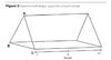
A graphical depiction of the mixture design experiments that would allow the calculation of a quadratic predictive equation for three ingredients is given in Figure 2.

The results of a quadratic mixture design can be quantified in a predictive equation. The equation, for three Y ingredients, is given in Equation 2.

Property (Y) = b1Y1 + b2Y2 + b3Y3 + b12Y1Y2 + b13Y1Y3 + b23Y2Y3 (2)

The design space in Figure 2 has each of the ingredients ranging from 0 to 100%. Mixture designs do not have to cover the complete design space; an ingredient might be varied from 50 to 100% or from only 20 to 30%, for example.

Crossed Designs

What does the researcher do when both factorial and mixture variables are present? I have seen colleagues optimize a formulation and then study process variables with the optimized formulation. This scenario means that a mixture design was done, a regression was completed and a response surface was plotted to get the optimized formulation. Then a process study was done on the optimized formulation. This unsuccessful methodology will be discussed later.

An alternative is to use a crossed design. The predictive mathematical model is obtained by multiplying the factorial equation by the mixture equation. The resulting no-intercept mathematical model is shown in Equation 3.

Property(X,Y) = Property(X)

A "Simple" Example

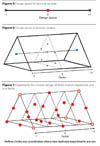
To illustrate how a crossed design is run, an experiment with three mixture variables, which each range from 0 to 100%, will be crossed with one factorial variable,5 which will use a coded variable from -1 to +1 with 0 center point.6 In this case, the experimental space can be drawn and is shown in Figure 3.

Normally what a researcher might do is first study the ingredient variables and develop an "optimized" formulation.

Let's say the researcher set the process factorial variable at "0." The researcher then did a very nice mixture design from 0 to 100 parts of each ingredient and found that the maximum property was 50 at 1/3 of each ingredient. For example, the response surface with the optimized formulation (red dot) is given in Figure 4.

Then very diligently, the researcher would take this optimized formulation and study the effect of the factorial variable by varying the factorial variable over the range of -1 to 1. The factorial design is one dimensional and is plotted in Figure 5, where the blue squares are the additional experiments combined with the center point of the mixture design.

If the design space of Figure 4 is combined with that of Figure 5, the new design space is shown in Figure 6. The experiments that the researcher ran are indicated in Figure 6. The red and green circles indicate the experiments run from the mixture design. (Coincidentally, the red circle represents the optimized formulation.) The blue squares represent the additional experiments run for the factorial design.

The researcher found that the property was still 90 at -1, but was 52 at +1. The researcher would be very excited, because the process study gave an increased value. But would he have the maximum property over the design space as shown in Figure 6? Look at all the design space that went untested. The researcher could find the optimum combination of mixture ingredients and process conditions, if he would run a crossed design.

For the design space represented in Figure 3, the predictive full quadratic model would be as shown in Equation 5.

Property (X,Y) = Property (X)

From the ANOVA, the important effects with >95% significance are A, B, C, AD, BD, CD, AD2, CD2, ABD and ABD2. The lack-of-fit is insignificant. A predictive equation can be defined using the coefficients in the ANOVA table as shown in Equation 6.

Property (X,Y) = 45A + 60B + 50C - 10AD - 20BD - 19CD - 20ABD + 16AD2 + 17CD2 + 69ABD2 (6)

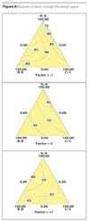
The easiest way to understand the results is graphically. Figure 8 shows slices through the design space at the Factor equal to -1, 0 and +1.

The question was whether the researcher found the maximum property by doing a mixture design at the midpoint of the factorial variable first and then using the formulation to study the factorial variable. The researcher had found a value of about 90 doing the work in two steps, which was a very good result. However, using a crossed design, the graphs show that a value of 99.8+ would be found. A triumph for statistically designed experimentation using crossed designs.

A Complicated Example

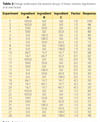
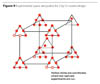
Let's consider what a design would look like if three mixture variables and three process variables would be studied. In this case, if a quadratic mixture model and a traditional two-level, full factorial design with center points were considered, 42 experiments would be needed to define the coefficients, five more duplicate experiments would be needed for error determination and five additional points would be run to determine factorial lack-of-fit. The D-optimal candidate set would be defined with 10 mixture experiments at each vertex and the center, or a total of 90 possible experiments. The statistical software would calculate D statistics to find the optimal 52 experiments. Figure 9 is a graph of the experiments chosen for the D-optimal design. The selection of the optimal experiments for the design is not intuitive or logical. I would have chosen a symmetrical design, but that is not the world of statistically generated design.8

After the experiments are run, the data would be analyzed and a triangle graph would be plotted for each of the factorial corners and center to understand how the property changes over the design space. For a design of this complexity, an optimization routine in analysis software should be used to find the coordinates of the optimum point.

Summarizing Thoughts

Crossed designs are not entered into lightly. The designs require a lot of experiments to be run. Once complete, however, the researcher can be assured that the one and only right answer will be obtained. This, in the long run, will save time, money and effort.