During presentations concerning averages and standard deviations in my short course, inevitably someone asks about outliers. Eventually I added a section about how to use the Grubbs Test to discern if a point separated from the body of data could be discarded. (1) But just what are outliers? Workers will judge a set of data and arbitrarily throw a point away that “doesn’t look right.” A dictionary definition is “a statistical observation that is markedly different in value from the others of the sample.” In sample data from a population, the outlier may be a datum that is higher or lower than the other data; or, several outliers could be higher and/or lower than the body of data.

Why do Outliers Occur?

Sometimes outliers occur because of human error. For example, a measurement is written into a notebook as 800 instead of the correct 80.0. Most times when an outlier is present, the researcher completes the experiment and records the data properly, but when the data is examined one or more data points just don’t seem to fit with the rest of the data.

William Kruskal wrote a short essay on wild observations, or, in our terms, outliers.(2) Kruskal remarked that if an outlier is identified, it must not be thrown away in a cavalier fashion. The outlier must be reported with the rest of the data and then be excluded from the overall analysis with a sound reason presented. One reason for exclusion is that the researcher knows for certain that the experimental run had a flaw in it. The flaw might be discerned before the experiment is over, e.g., a resin overheats, or after, e.g., the notebook might document that the wrong procedure was used. Sometimes the outlier can’t be explained. The usual practice is to exclude the outlier on the basis of some statistical test. If the suspect data point is excluded, the exclusion should be done reluctantly and the analysis of the remaining data should be done with great caution. In any case, to repeat, all of the data should be reported, the outlier should be identified and a reason be given as to why the outlier was excluded.

How to Detect Outliers?

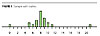
Use of a graphical method such as dot diagram or histogram is a good way to identify a possible outlier (see Figure 1, the histogram of the data in Table 1).

When the sample size is small, e.g., three samples giving readings of 3, 4 and 12, the researcher may decide out-of-hand to discard the 12 because it is not close to the other two, which match pretty well. But this is dangerous, because the range of results might only be due to normal experimental variation. The researcher should run more replicates.

For regressions, a plot of the data may show an outlier (Figure 2). Diagnostic statistics can give a hint whether the suspected outlier should be ignored when the data is analyzed. The plot shows that point 16 is suspect and should be closely examined. We’ll discuss regressions in a future article.

Statistical Testing for Outliers in a Population

After a decision has been made that an observation is a possible outlier and no rational explanation exists why the observation should be excluded, the researcher, with trepidation, can turn to one or more statistical tests. Some are simple; some are not. A short list of these will now be discussed. Other tests exist, but these give a range of methods.

Plus/Minus Standard Deviations
A simple test is to determine how far the outlier is away from the average in terms of standard deviations. The Bienaymé-Chebyshev inequality (3) says that the probability of a point being within k standard deviations (s) of the mean is 1/k2. So, for example, the decision to discard an observation that is + 4s is not bad, since an outlier which is > 4s distant from the mean occurs less than 1 time in 16. This test works best with a sample size of at least ten, and the greater the number of points the better.

Example 1

The data set of Table 1 has an average of 8.2 and standard deviation of 3.6. If a data point that is 4s greater than the average, the exclusion limit would be 8.2 + (4 * 3.6) = 22.6. Since the suspected outlier has a value of 21, the suspected outlier cannot be discarded using this test. If a 3s test was used, the exclusion limit would be 8.2 + (3 * 3.6) = 19.0, and the suspected outlier could be discarded. The danger is that the researcher would be wrong to discard the point 1 time in 9, not very good odds.

The Grubbs Test
The Grubbs Test (4) formalizes the standard deviation test and compares the calculated result, Q, to a set of statistics by using the following equation:



                | average minus possible outlier |
Q  =   ----------------            (1)
               Standard Deviation of Data Set
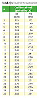
The absolute value of the difference between the sample average and the suspected outlier is used since the outlier could be smaller or larger than the data set average. Dividing this difference by the standard deviation gives Q. The calculated Q is compared to the Q statistic in Table 2 using the number of observations in the total data set and the appropriate column of probability.

Example 2

The data set of Table 1 has an average of 8.2 and standard deviation of 3.6. Run number 14 with a result of 21 looks to be an outlier. The information is substituted into the Grubbs equation and the Q statistic is calculated.

               | 8.2 – 21 |              12.8
Q  =   -------  =  -------  =  3.6
               3.6               3.6
A comparison of the calculated Q value to the Q value in the table with n = 22 shows that the suspected outlier could be excluded with > 98% confidence (a < 0.02), which means the decision to exclude the data point would be wrong less than 2 times out of 100. Using the Grubbs test the outlier is removed and the average would be recalculated and reported as 7.6. The standard deviation would now be 2.3. Remember, all 22 data points should be reported and the rational given for discarding the suspect observation.

Observation 22 is also suspected of being an outlier, but the Grubbs test can only be used once on a set of data.

Box Plot
Tukey (5) developed a graphical method to display sample data, the Box Plot. A Box Plot, illustrated in Figure 3, shows the data of Figure 1. The Box Plot portrays several different statistics as well as any outlier points. The box itself portrays the lower bound of the second quartile and the upper limit of the third quartile based on the count of data. A line inside the box indicates the median of the observations. Whiskers extend from the top and the bottom of the box, which indicate the minimum and maximum data values, unless an outlier is present and the whiskers are then 1.5 the length of the quartiles. The width of the box is 1.5 times the log of the number of points, which may be useful if comparing several different samples with different numbers of observations. Possible outliers are also indicated. Although not from Tukey, a diamond diagram may also be included. The side points of the diamond indicate the average, while the top and bottom points of the diamond indicate the standard deviation.

Dixon Test
The Dixon Test is based on the ratio of ranges of ordered data, so that normally distributed data is not required. (6) The test performs well with small sample sizes.

The data is sorted either in ascending or descending order with x1 being the suspected outlier. Then a ratio, R, is calculated from the ranges of x1 to x2 and of x1 to xn.

               | x1 – x2 |
R  =   ----------  (2)
               | x1 – xn |
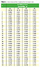
The decision to exclude x1 as an outlier is made by a comparison of the calculated R statistic to a list of critical values. The critical values for R, given in Table 3, are used when n is 3 to 7. Applicable tables of R statistics are available when n is 8 to 10, when n is 11 to 13 and when n is 14 to 30.

Example 3

The 22 data points of Table 1 were ordered with the suspect outlier listed first: 21, 11, 10, 10, 9, …, 5, 5, 0. The Dixon ratio was calculated.

               | 21 – 11 |               10
R  =   -----  =  -----  =  0.476
               | 21 – 0 |                  21
A comparison of the calculated R value to the R statistics with n = 22 in the table shows that the suspected outlier could be excluded with > 99% confidence (a < 0.01), which means the decision would be wrong less than 1 time in 100. The outlier is removed and the average would be recalculated and reported as 7.6 and the standard deviation would be 2.3. Remember, all 22 data points should be reported and the rational given for discarding the suspect observation.

Pierce Criterion
In the previous outlier tests, only one outlier could be removed. The Pierce Criterion, as described by Ross, (7) allows for the sequential elimination of one or more suspected outliers, whether they all high, all low or maybe some are high and some are low.

Example 4

The data in Table 1 show two possible outliers - one high value, 21; and one low value, 0. The mean and standard deviation of the distribution are calculated to be 8.2 and 3.6, respectively. The value of P statistic for one doubtful observation for n = 22 from Table 4 is 2.251. The maximum allowable deviation for a data point that belongs to the data set is 3.6 * 2.251 = 8.1. The deviation for the first suspected value is |21.0 – 8.2| = 12.8. This deviation is greater than the maximum allowable deviation of 8.1 and the corresponding outlier point of 21 is removed from the data set. Since a second point is a possible outlier, the process is repeated using the statistic for two doubtful observations. The R statistic from the table for n = 22 and 2 doubtful observations gives 1.960. The maximum allowable deviation is 3.6 * 1.960 = 7.1. The deviation of the second most outlier point is |0 – 8.2| = 8.2 which is greater than 7.1 and so the second outlier point is rejected. If additional doubtful observations are present the process would be repeated until the deviation of a point from the mean is less than the calculated maximum allowable deviation. All 22 data points should be documented and the rational given for discarding the suspect observation. The average and standard deviation of the remaining eighteen remaining points should be reported as the values found for the experiment.

Hampel’s Method
The Hampel method results in a score8 that is based on robust statistics, and makes use of the median, which is more robust than the mean. When the mean and standard deviation are used for determination of outliers, as in the Grubb’s Test, the outlier will affect the result. For example, an outlier is on the high side of the average; when it is discarded both the average and standard deviation become smaller. When the median and the median of the absolute deviation are used and the outlier is discarded, the median and median of the absolute deviation will usually remain the same. Also, in contrast to other tests, where only one outlier can be discarded or the outliers are discarded sequentially, the Hampel method makes no assumption on the potential outlier(s).

The median is computed from all the values, and, then, the absolute deviations (residuals) between the experimental values and the median are computed. A median of the absolute deviations (MAD) is then determined. The value of 1.48 × MAD is used as a robust estimate of the dispersion of the values from the median. The Hampel Score, H, is calculated using the following equation.

H = (xi – median) / MAD               (3)

Usually, xi is considered as an outlier when H is greater than some cut-off statistic. Use of H = 2.5 is very liberal in excluding outliers. A more robust test would be if H is 4 or 5. Hampel recommended that H should be greater than 4.5.

Example 5

The data from Table 1 will be used to demonstrate the use of the Hampel Score. The median of the 22 data points is 8. The absolute deviation of each data point is calculated by subtracting the median value from each data point, | (xi – median) |. The median of the absolute deviations is 3. Finally, H is calculated by dividing the absolute deviation by the median absolute deviation. a review of the Hampel scores reveals that Experiment 14 has H = 4.3, probably an outlier; and Experiment 0 has H = 2.63, probably suspect, but maybe should not be discarded without an additional reason.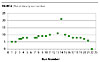

Do Outliers Lie?

As mentioned above, the researcher must be careful when considering a data set. Diagnostic statistics assume that the data is distributed normally, that is, the replicates follow a normal distribution – experimental variation is just as likely to give a value above the true value as below the true value. In some instances this is not the case. For example, tensile strength tends to have more values on the low side of the average than on the high side. Defects in samples cause premature rupture of the sample. Tensile strength data sets may look like the following: 2800, 2850, 2750, 3800. I have seen researchers discard the 3800 value, because a statistical test told them to do so. The sample with a value of 3800 is most likely to be close to the true value, with the other values coming from premature failure.

Another example is rusting in corrosion prevention coatings. A researcher diligently characterizes the rust resistance of duplicate panels and gets surface rust of 10 and 25% of the original after five thousand hours of immersion in salt water. The researcher computes and reports the average and standard deviation. Corrosion testing is similar to tensile strength, in that the experimental variation is not normally distributed. Test results tend to give more points with high failure and fewer with low failure. One possible cause is the presence of pinholes, which allow the salt water to get to the panel surface. The panel with 25% rust is likely not to be indicative of how the coating performs, but rather an indication of how well the panel was prepared. In skewed tests like these examples, the way to get better results is to run more replicates.

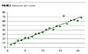
The data of Figure 1 is actually process data grouped by the value of the response. When the data in Figure 1 were plotted in the order the measurements were taken (Figure 4), the potential outliers now look like an indication of a process problem and cannot be excluded from the data set.

Outliers as Inventions

Sometimes the researcher uses statistical design in a carefree, heedless manner looking at the numerical data and doing statistical tests without really looking at the test specimens. An illustration of this happened to me when I evaluated the gloss retention of polyurethane coatings based on acrylic polyols. Three polyols with varying physical and drying properties were to be blended. The idea was to use these as blending partners to get intermediate properties. Individually, each resin gave coatings that had three year Florida gloss retention of about 50% of the original gloss and confirmation was desired that the blends retained this quality.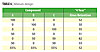

A three ingredient, mixture design was set up with each ingredient varying from 0 to 100%. Table 6 gives the design and the gloss retention after the coatings were prepared and exposed to accelerated weathering to simulate four year Florida exposure,

All the coatings made with the blends except one were in the same range as the coatings made with the pure components. The inclination would be to say that the one point was an outlier and report that the blends could successfully be used. Initially that is what we did. But when we reexamined the panels and the data, we found an unexpected synergism with the blend of Components B and C. As good researchers, we replicated this formulation. The same high gloss retention was reproduced. Moreover, when the acrylate monomers of Component B were combined with those of Component C and then polymerized, the gloss retention of the new acrylic polyol was just as good and lead to a new product Component D. This resulted in two new patents: one for the physical blend and one for the new polymer made with the monomer blend. Not a bad months work.

Conclusion

The moral of the story is that researchers should be on the lookout for the outlier that will lead to the next discovery and invention. You don’t want to be the researcher that discards an invention. The safest thing to do would be to run additional replicates of the outlier experiment.