Editor's Note: This article is Part 8 in a series. See PCI October 2002 for the previous installment.

The previous article initiated a discussion on factorial experiments. The article concentrated on full factorial experiments where all combinations of every level of all variables are tested. For example, if four variables were to be evaluated at four levels, 256 experiments would have to be done. When continuous variables are studied, two level full factorial designs with center points can be used to minimize the number of experiments; for example, four variables can be studied at two levels and would require 16 experiments and five center points. Using only a fraction of the full factorial experiments can have further savings. This article begins a discussion on fractional factorial designs, but I'm going to come from a different direction.

A Practical Example

Let's consider a real-life example. A latex paint manufacturer has four formulations. He wants to know if the formulations have the same or different dry times.

The experimental factor of interest is the four different formulations. The response or test of interest is the dry time.

Other variables may affect the dry times during our experimental runs. These are sometimes termed nuisance factors. A researcher must decide whether to hold the nuisance factors constant, e.g., using a constant temperature and humidity room, or to purposely vary them to determine their effect. A third choice is to hold some of the less interesting nuisance factors constant and to vary the more interesting ones. For the dry-time measurement, nuisance factors could be the dry-time meter, the order of the experiments, the temperature, the humidity, the film thickness and different operators.

Finally, the researcher must realize that any number that is measured will have random variation1 associated with it. In other words, if a researcher repeats a test exactly by holding everything in his control constant, random variation will be part of the measurement and give different results for replicate experiments.2 Random variation is generally reported as the standard deviation.

Now the researcher needs a well-designed experiment.

What is a Bad Design Compared to a Good Design?

Sad to say, in most labs a single measurement is made for each paint and then the results are compared. This is illustrated in Figure 1, where each box represents a separate experiment and each shade represents a different paint formulation. The dry times were determined at the same time using four different timers.

When a single experiment is run, the operator really doesn't know if differences are caused by the different paint formulations or by experimental variation (and experimental variation is present in all data measurements). This experiment is doubly bad, since, if no experimental variation is assumed (like most labs), the operator doesn't know if different dry times are due to the different paint formulation or due to the different timers.

To take care of the experimental variation, an experienced researcher knows that replicates must be run. The number of replicates needed depends on how much experimental variation is present and the difference in a property that is significant (see "deSigns of the Times: Or, t-ing off," PCI September 2000). If experimental variation is high or if detection of small differences in a property is important, many replicates may be needed.

Figure 2 illustrates one possible design, where four replicates were run.

In this case, if a difference in the dry times is seen, the operator can be confident that the difference is real. However, he still doesn't know if the difference is due to the formulations or if the difference is due to a difference in dry-time meters.

A better design strategy would be to randomize the runs using different paint formulations with four different dry-time meters. This is illustrated in Figure 3. Series 1 was run; then Series 2, etc.

Experimental variation caused by the dry-time meters is spread over all the paint formulations. Now the differences between paint formulations could be determined. A close examination of Figure 3 reveals that in two cases the same dry-time meter was used for the same paint formulation. An improved scenario would ensure that each paint formulation would use each dry-time meter only once. This would be an example of a full factorial design with 16 experiments. Not only can differences between paint formulations be determined, but also differences between dry-time meters. One possible design scheme is given in Figure 4.

One further difficulty is that the experiments cannot all be done at the same time. In effect, a new variable is added, that of time. In Series 1 of Figure 4 the same formulation was used in two of the runs; this was also the case in Series 2 and 3. This could lead to an erroneous conclusion, if, for example, the temperature or the humidity in the lab changed.

A full factorial design with four paint formulations, four timers and four run times would amount to 64 experiments. A fractional factorial design of 16 experiments is given in Figure 5. This design allows not only the identification of the differences in dry times due to the different formulations and different timers, but also any difference in dry times over the course of the experiments. This is known as a fractional factorial design, because only 1/4th of the 64 possible combinations is run.

A close examination shows that for each experiment (as designated by each square), a unique combination of column, row and color can be listed. For example, the square in the first row and column can be coded "row 1, column 1, color white". This coding is not repeated for any other square. This symmetrical, experimental design goes by the name of "Latin square." The Latin square of Figure 5 goes by the designation of a 4 x 4 x 4 design. Latin squares can be constructed for more or fewer variables. Examples are shown in Figure 6.

Using a Latin square and Analysis of Variance or ANOVA (see "deSigns of the Times: Or, When an F is a passing grade" PCI August 2001) all of the necessary information about the individual factors and the level of each factor can be gathered in a fraction of the experiments.

One constraint for using Latin square designs is that no interaction occurs between variables. That is, no combination will give an unexpected synergistic response that wouldn't be predicted from the individual variables. In the example, a researcher would have no reason to believe that an interaction would occur between the paint formulation and the timer, between the paint formulation and the measurement day or between the timer and the measurement day. If an interaction did exist, a condition of confounding would exist that would cast doubt on the results. If an interaction were suspected, then additional experiments would have to be run.

Latin square designs are especially useful for categorical variables to distinguish which variable was statically distinguishable from the others and which level of the statistically significant variable was different from the others. If continuous variables were to be studied, a better design would be a two level design with midpoints that would have only 12 experiments; or, if quadratic components were present, the choice would be a central composite design with 18 experiments.

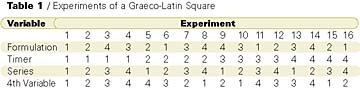
If an additional variable is to be studied, it can be added to the Latin square shown in Figure 5. This hyper-Latin square is sometimes termed a Graeco-Latin square. The four-factor design is shown in Figure 7. Again, each square has a unique combination of column, row, color and letter. The experiments showing the 16 unique combinations of Figure 7 are given in Table 1 using codes for the four levels of each variable.

A full factorial design with four variables, each at four levels, would contain 256 experiments. The factorial design, given in Figure 7 and Table 1, is also known as a fractional design because only 1/16th of the 256 possible combinations is run.

Use of a Latin Square in Paint Formulation

In the real life example, the factor of interest was different formulations of latex paint. The response to be determined was dry time. Nuisance factors included different timers, temperature and humidity, measurement time and film thickness.

Random variation occurred when the research measured the results using the dry time template. Dry time is determined by the use of a small clock with a stylus attached to a single minute hand. The stylus draws a line in the wet paint. Initially, the stylus digs all the way to the substrate. When the paint is "set to touch" the stylus rides up on the paint but still gauges a line. When the paint is "surface dry" the stylus no longer gauges a line, but still mars the surface. The paint is "hard dry" when the stylus leaves no mark.

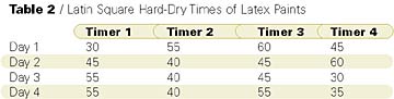
The researcher decided to use the Graeco-Latin square shown in Figure 7. Four formulations, four dry-time meters and four film thicknesses from 1.0 to 1.75 mil were to be evaluated over four days. The determinations would be made in a constant temperature and humidity room. The results are shown in Table 2. Averages can be calculated for each level of each factor and are shown in Table 3.

A danger at this point is to take the averages at face value. The researcher needs to construct an ANOVA table to determine whether the differences are real or are due to random variation. The ANOVA is shown in Table 4. df is the degrees of freedom: three because each factor had four levels; SS is the sum of the squares; MS is the mean square (SS divided by df) or variance; and F is calculated by dividing the MS for each factor by error MS). The Probability is estimated by comparing the calculated F in Table 4 to the F values found in a statistics reference. The square root of the error MS is the standard deviation for the experiment: 1.25.

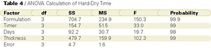
The ANOVA table shows that with >99.9% probability the different formulations had different dry times; with >99% probability the different timers had different dry times; with >98% probability the different days had different dry times; and with >99% probability the different thicknesses had different dry times.

Taking experimental variation into account, the question is "Which level of each factor is different than the others?" Using the standard deviation, any two levels that have dry times different than about three minutes have statistically different dry times. Two levels that are less than three minutes are statistically indistinguishable.

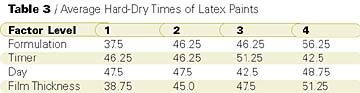
A review of Table 3 concludes that Formulation 1 has the fastest dry time, while Formulation 4 has the slowest; that dry-time meter 3 reported the slowest dry times, while dry-time meter 4 had the fastest; that Day 3 had the slowest times (maybe due to a malfunction of the air conditioning equipment); and that as film thickness increased the dry time became longer.

Other Types of Fractional Factorial Designs

The Latin square is just one example of a fractional factorial design. One example is a two-level design that is used for screening and optimization experiments that define mathematical relationships. Other designs include the Plackett-Burman designs, which are set designs used in screening large number of variables; the Box-Behnken design, which is useful when interactions are known to be present; and the D-Optimal design, which allows the least number of experiment to be run when the mathematical relationship is known. These can be the topic of another article.