Editor's Note: This article is Part 6 in a series. See PCI August 2001 for the previous installment.

In the first five articles, the basis for statistical inference was discussed in terms of experimental variation and statistical testing involving the t and F statistics. The next articles will discuss strategies for the selection of experiments by a statistically minded researcher. This article describes some initial considerations.

Mathematical Relationships

In research and manufacture, data is often generated by changing some conditions and then measuring the result. This relationship is often expressed mathematically and graphically. Mathematical analysis is called regression analysis and graphical depictions are known as regression plots.1

In regression, there are two types of variables: independent variables, which the researcher chooses to study and set at specific limits; and dependent variables, which the researcher measures as the result of the test. Usually the independent variable is plotted on the X axis and the dependent variable is plotted on the Y axis. As with all data, error is associated with setting the independent variable and measuring the dependent variable. This results in uncertainty in the graph, so that the statistically minded researcher will also plot the 90%, 95% and 99% confidence limits.2

A typical regression with confidence limits is shown in Figure 1. The plot was made from duplicate data taken at five positions along the X axis. The regression and confidence limits were calculated using a least squares calculation. Y can be predicted for any desired X. For example, if the dependent variable were to be predicted at X = 12, the researcher would not say that the predicted value would be 140. Rather, the researcher could say that the predicted value of the dependent variable would lie within the range of 120-160 with 90% confidence. That is, the researcher would be wrong only one time in 10, i.e., with 90% confidence, when he says Y will be somewhere between 120 and 160. At the ends of the plot the confidence range gets larger, because experimental uncertainty is greater. In an equation like Y = a + b * X, there is uncertainty in both the intercept a and the slope b. Of course, with increasing confidence the prediction range gets larger.

How Is a Mathematical Model Selected?

Many researchers take data and then try adding X terms to the equation until an acceptable regression is formed. If enough terms are added, a perfect regression is obtained every time. The danger is that the equation will be meaningless and will have little value in predicting intermediate values.

Statistical methodology requires that an experimental hypothesis be put forth before data is gathered, and that experimentation is planned in order to disprove the hypothesis.3 Similarly, when a researcher is required to define a response equation, he must put forth a hypothetical mathematical equation or model and then try to disprove it with properly chosen experiments.

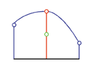
Predictive models often are not simple. Figure 2 shows a very complex response curve, maybe a cubic hypersine or some such. However, if the experimental region is limited the mathematical model can be simplified. For example, if the range of the independent variable is limited to that as defined by A, the model would be a linear equation. If data is collected over the range of B, C or D, a simple quadratic equation would define the models for these ranges.

Proper planning can prevent curvature from being present in the design space being studied. For example, if the experimental range is very narrow, models for the design space are almost always linear. The danger is that experimental ranges are too narrow and important results will be missed.

I was told by an applied statistician that usually 80% of all experimental data will be fit by a linear model, i.e., linear independent variable terms like a1X1, a2X2 and a3X3; another 10% of data would require a second order model, i.e., interaction and square terms like a12X1X2 and a11X12; and another 5% would require a third order model, i.e., interaction and cubic terms like a123X1X2X3, a112X12X2 and a222X23. The last 5% of all data requires special terms, e.g., reciprocal, a1/ X1. A hypothetical model might look like that in Equation 1.

The objective for the researcher would be to define experiments that would disprove this equation. If he could not disprove it, he would accept it as true until which time more data might disprove it.

If the equation is complicated, involving logarithmic or trigonometric functions (see Equation 2), a simple equation can still be defined by use of a substitution.

If the researcher substitutes s = log y and t = sin(x) , then Equation 2 becomes Equation 3, which is a simple quadratic equation.

When curvature is present, second or third order terms must be included in the equation. Statistically designed experimentation that tests for these higher terms have more experiments than when only linear terms are present. In general, one experiment must be performed for each term in the hypothetical equation.

How Are Experiments Statistically Selected?

Now that a hypothetical model has been proposed, experiments can't be chosen willy-nilly, but rather according to a special plan. Experiments are chosen that would disprove that the terms in the model are significant. In addition, additional experiments are included that could disprove the hypothesis that the proposed terms are the only viable ones.

If an experimenter is uncertain what result will be achieved under a given set of experimental conditions, he runs the experiment to reduce his uncertainty. If his uncertainty is high for other conditions he runs an experiment in that area. He continues to run experiments where he is most uncertain, that is, where there is the most error.

Where is the most uncertainty for the plot in Figure 1? At the ends of the model. Experiments run at the extremes of the experimental conditions have more leverage than those near the middle, just as a person has more leverage by grabbing the ends of a stick vs. having both hands in the middle. When I was in college I was taught to evenly space out my experiments, even when I expected a straight line (see Figure 3A). This gave me a lot of information about the experimental variation in the middle of the line but not much information about the ends. If I know absolutely, that I am studying a linear model, leverage suggests that a better design would be to run the same number of experiments at the end of the design space (see Figure 3B).

Both of the regressions 3A and 3B have the same amount of error in the Y coordinate, and so the intercept; however, because of leverage, the error in the slope is less in B than in A. If the experiments can be moved slightly further apart, even less error would be seen in the slope (see Figure 3C). The experimenter must be careful not to move the experiments too far apart or the experiments might be in a region of curvature, and this design will not detect that.

The experimenter can interpolate these results; that is make predictions within the experimental design. However, he should not extrapolate beyond the experiments, at least not very far, because there could be curvature beyond the experimental boundaries.

In order for the experimenter to disprove the hypothesis that the model does not have higher order - square or cubic, etc. - terms, he must include several experiments to test "lack-of-fit." In a basic design, the first experiments chosen are at the ends of the experimental region (see Figure 4A). If the experimenter wants to determine if terms of a higher order are present, the coordinate with the most leverage for second order terms is the experiment in the middle of the design space-the mid-point (see Figure 4B). The best coordinates for testing for the presence of third order terms are at the one third and two thirds points (see Figure 4C).

If the experimenter proposes that the regression is linear and the proposition is true, the results of the experiments at the mid-points would fall on the dashed line; if the proposition is false the mid-points would fall off the dashed line. This reasoning also holds for testing cubic models. The design in Figure 4C would also test a quadratic hypothesis but requires additional experimentation. As reported above cubic models are rare unless the design space is large. The usual practice is to include only center points when designing the experiments.

To balance experimental "power" with experimental economy, four or five replicates are required for each level of the design.4 Figure 5 shows the distribution of experiments over the design space (the Xs or independent variables) of statistically designed experiments for one, two and three variables.

In Figure 5A, the one variable design, four experiments are chosen at each end of the design space and four experiments are chosen in the middle to test for lack of fit for higher mathematical terms. In Figure 5B, the two variable design, two experiments are chosen at the corners of the design and four are in the middle. Why are two experiments chosen at each corner? The experiments on the left side of the design are all done at the lower level of the first variable, while those on the right side are done at the high level. The result is running four experiments at each level. Similarly, the experiments on the bottom of the design are run at the low level of the second variable, while those on the top are done at the high level of the second variable - again, four experiments at each level. In Figure 5C, the three variable design, only one experiment is done at each corner and four done in the middle. Again the experiments on the left side of the design are all done at the lower level of the first variable, while those on the right side are done at the high level. The result is running four experiments at each level. The experiments on the bottom of the design are run at the low level of the second variable, while those on the top are done at the high level of the second variable - again, four experiments at each level. The experiments on the front of the design are run at the low level of the third variable, while those on the back are done at the high level of the third variable - again, four experiments at each level.

For the experimental designs of Figure 5, the four experiments at each level, horizontally, vertically or front-to-back, are averaged to get an estimate of the response at that level. Independent estimates of each variable can be made, because in a balanced design, the changes in the other variables are uniform and cancel out.

An example for a three factor design is given in Figure 6, where the experimental result for each corner is plotted. The values of the front - 3, 2, 5 and 4 - give an average response of 3.5; and the values of the back - 4, 3, 6 and 5 - give an average response of 4.5. Similarly, the values of the left are averaged to give a value of 4.5; and the values of the right give 3.5. Finally, the values of the bottom are averaged to give a value of 3; and the top give 5.

In summary, running experiments at the corners of the design space as in Figures 5B and 5C gives sufficient information on the linear terms, e.g., X1 or X2, and any cross-product terms, e.g., X1X2, so that a mathematical model can be constructed. For example, see Equation 4 for the two factor model and Equation 5 for the three factor model.

The end point experiments are not sufficient to judge whether quadratic or cubic terms are needed. For this the midpoint experiments must be evaluated.

How Are the Midpoints Used to Judge for Higher Order Terms?

The presence of higher order terms is determined by use of a t-test.4 A t-test requires two averages to compare. All the experiments for all the end points are averaged as an estimate of the result for the mid-point. Then the end point average is compared to the actual results determined at the mid-point using a t-test. For example, Figure 7 shows experiments with the results plotted as balls on the vertical axis.

In the one factor example of Figure 6A, the values for the balls on the ends of the line are averaged to get a value for the mid-point that resides on the line. This calculated value is compared to the real value for the mid-point, shown as a ball on top of a stick going through the mid-point, using the t-test. Similarly, for the two factor example of Figure 6B, the values for the balls on the corners of the square are averaged to get a value for the mid-point of the plane. This calculated value is compared to the real value for the midpoint, shown as a ball on top of a stick going through the middle of the plane, again using the t-test.

Using the data of Figure 6, an overall average of the eight points is 4. If the average of the four center point experiments were 4, a conclusion would be that there were no higher order terms present. But, if the average of the four center points were 8, a conclusion might be that one or more of the three factors required a higher order term in the mathematical model.

For a single variable experiment, like that in Figure 5A, the experiments provide enough information to estimate the quadratic coefficient (see Figure 8).

However, when two or more variables are present, if a higher order term is present, the experiment can't tell which variable is responsible. One or more higher order terms might be required (see Figure 9).

When the experimenter has shown that the model must include higher order terms, the current data cannot tell him what it should be. The experimenter must do additional experiments to distinguish which variable or variables need higher order terms. The additional experiments fall between the ends of the initial experiments. Figure 10 shows the original square design space with the additional experiments. Compare to the original design in Figure 5B.

The new experiments fall on a square just like the original design (Figure 5B) but which has been rotated 45degrees from the original design. These are called star points. Typically, at least duplicates, as shown, are run. As it turns out, the experiments from the end points of the original design and the new experiments on the star points fall on a circle. Four new mid-points are included in the second round of experiments to test for changes that may have occurred between the times of the two designs. The new data is combined with the original data and the full quadratic model, including square terms, can be determined.

Designs with three or more factors are treated the same way, but it's hard to draw in more than two dimensions.

Are there Other Considerations in Experimentation?

For statistically designed experimentation to work properly, it is assumed that error is random. In order for this to be so, experiments must be done in random order. For example the experiments of a three variable design in Table 1 are listed in standard order; one possible random run order is listed. (Statisticians normally code the levels of the variables. Instead of saying that the low level of a temperature variable will be 100degrees and the high level will be 150degrees, the statistician will use codes of -1 for the low level and +1 for the high level. This is done to make all the calculations homogenous if the variables don't use numbers of similar magnitude. This coding is used in Table 1.)

Experiments are run in random order to prevent unwanted "blocking " of experiments. Variable C has all of the -1 level in the first four experiments and all the 1 level in the last four. Suppose two lots of resin are being evaluated over a two-day period using standard order. One lot is assigned the -1 level with its experiments run the first day and the other is assigned the 1 level with its experiments run the second day. What if something happens overnight, perhaps the temperature in the lab changes by 10?. Now the first lot is run at a different temperature than the second lot, and the results are confused or "confounded." The experimenter doesn't know if a difference in results is due to the difference between the lots or between the temperatures. If the experiments had been run randomly, the temperature change would have been spread out between the two lots.

Sometimes experiments can't be run on the same day and blocking is purposely invoked to separate the variation due to the different days. A fourth variable is defined as the day the experiment was conducted in order to determine the day variance.

Final Considerations

When a researcher decides to use statistically designed experimentation, he commits to doing as many experimental designs as are needed to get the results. In some cases, the first design will be enough, if no higher order terms are present. If higher order terms are present, additional experiments are required. Statistically designed experimentation will provide a pathway to get the goal in the most efficient manner.