deSigns of the Times: Slacking Off!
Editor’s Note: This article is Part 14 in a series; see PCI, March 2007, for the previous installment.
In previous articles1,2 factorial designs were described as being especially well suited to studying continuous variables, like pressure, temperature, time and speed, and categorical variables, like chemical functionality type, lot number and position. Mixture designs were described as being especially suited to studying variables that add to 1 or 100%, like blends, formulations, reactions, oligomers and polymers.
I have a colleague who has a Ph.D. in applied statistics and champions experimental design wherever he can, but has never used mixture statistics. When a mixture design is called for, he refers his clients to me. Before he knew me (and even now when he thinks he can get away with it), whenever he had a mixture to study, he used a slack-variable, factorial design.
This article discusses the differences between a slack-variable, factorial design and a mixture design.

0.30 ≤ A ≤ 0.40
0.30 ≤ B ≤ 0.40
0.30 ≤ C ≤ 0.40
If a standard factorial design was to be used, a low level, coded as -1, would be set for each variable at 0.30 and the high level, coded as +1, at 0.40. A three-factor, factorial design of this type is given in standard order in Table 1. A center point experiment is included, and experiments for estimating the quadratic coefficients are also included. The first columns for A, B and C are shown in the coded form; the second columns for A, B and C are shown with the actual levels of ingredients; and the third columns for A, B and C are shown with normalized levels of ingredients.
The levels have to be normalized because several of the sums of ingredients in several of the experiments do not total to 1. The sum of all ingredients has to total 1. Experiments 1, 11, 13 and 15 have ingredients that total less than 1. Experiments 4, 6, 7, 8, 10, 12 and 14 have ingredients that total more than 1.
Now new problems arise. After the experiments were normalized to 1, the first problem is that several experiments have normalized levels of ingredients below the desired 0.3.
Another problem is that Experiment 1 with the –1, –1, –1 coding has the same normalized levels as Experiment 8, with the +1, +1, +1 coding and Experiment 9, with the 0, 0, 0 coding. This prevents doing any meaningful mathematical analysis.

One issue is that the C variable falls outside of the desired experimental range. This is an artifact of the slack, factorial design. Hopefully the formulation with C as low as 0.2 will still work. If not, no data will be obtained for Experiments 4, 6 and 8, and no response surface analysis would be possible.
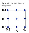 The star points normally lie outside the design range at –1.4 and +1.4 for each ingredient. However, the star point levels were adjusted to –1 and +1 since the design was not to be greater than the range of 0.3 to 0.4. The design space and design points are shown in Figure 1.
Assuming the researcher had data for all of the experiments, when the quadratic regression equation is analyzed for the factorial design using the experiments of Table 2 the equation would have the following form.
Property = b0 + bAA + bBB + bABAB + bAAA2 + bBBB2 (1)
 If all the coefficients were significant, one would interpret them by saying, for example, that when A is varied the Property is changed by aAA units and aAAA2 units. Similarly, when B is varied the Property is changed by aBB units and aBBB2 units. In addition of course, when either A or B is varied, one would also see a change in the contributions of the interaction term AB. What is seemingly lacking is what contribution C makes, since it is also being varied. An inexperienced researcher might ignore C’s contribution or assume it is non-existent. The effect of C is buried within the b coefficients, but more of this later.
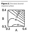
The response surface that is generated from the slack, factorial design data of Table 2 is given in Figure 2. The graph can be used to predict formulations that would give a specific result. For example, one formulation that would give a value of 90, would be when A = 0.35 and B = 0.40. Then C would have to be set to 0.25.

The experiments needed to define a quadratic mathematical mixture model are listed in Table 3. (I used the same response equation of the slack, factorial design to calculate the properties, so that a comparison can be made later.)
 The design points, along with the design limits, are shown in Figure 3. The design space in Figure 3 is bigger than it should be, so that later the mixture design space can be compared to that of the slack, factorial design space.
When the regression equation is analyzed for the mixture design it would have the following form.
Property = aAA + aBB + aCC + aABAB + aACAC + aBCBC (2)
If all the coefficients were significant, one would interpret them by saying, for example, when A is increased the Property is increased by aAA units. In addition of course, when A is increased either B or C or both are decreased and then the Property will be changed by the change in aBB and/or aCC. One would also see a change in the contributions of the interaction terms AB, AC and BC. The comments for increasing B or C would be similar.
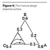 The response surface for the mixture design is shown in Figure 4.
Wait a minute! This response surface only has properties varying between from about 45 to 70. The slack, factorial design had performance varying between about 45 and 140. Let’s look at what is happening in the slack, factorial design.
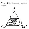 If the experiments do work, the response surface would be like that in Figure 6. The property range is from about 45 to 140, just as in Figure 2.
The mixture design response equation was given in Equation 2. As already stated, the following equality holds:
A + B + C = 1 (3)
Equation 3 can be rearranged to give the following:
C = 1 – A – B (4)
If C in Equation 2 is substituted with Equation 4, a slack equation is obtained:
Property = aC + (aA – aC + aAC)A + (aB – aC + aBC)B + (aAB – aAC – aBC)AB – aACA2 – aBCB2 (5)
If we compare Equation 5 to Equation 1 we see the following:
b0 = aC (6a)
bA = (aA – aC + aAC) (6b)
bB = (aB – aC + aBC) (6c)
bAA = – aAC (6d)
bBB = – aBC (6e)
Equations 6a through 6e show that the effect of C on the Property is contained within the b0, bA, bB, bAA and bBB coefficients. This means that Equations 1 and 2 are equivalent. That is, a plot of the response surface of Equation 1 has been shown to be equivalent to that of Equation 2.
In the past, when an unsophisticated researcher viewed an analysis of variance table from a slack experimental design, if the variable A showed a significant effect, the researcher would attribute the effect to a change in A as manifested by the magnitude of the bA coefficient. But, looking at Equation 6b, if the bA coefficient is significant, the researcher doesn’t know if it is due to an effect from the variable A, the variable C or their interaction, AC. Similarly for the B variable, if the bB coefficient is significant, the researcher doesn’t know if it is due to an effect from the variable B, the variable C or their interaction, BC. However, the researcher can get an idea of the magnitude of the effects of C, AC and BC, by looking at the coefficients of b0, bAA and bBB. Then the researcher can do some mental gymnastics to determine how much C, AC and BC contribute to the effect of A or B. To my mind it is easier to use the mixture equation of Equation 2.
Another point for why I favor mixture designs is that even for the simple example of three ingredients, the quadratic mixture design has fewer experiments than the quadratic-slack, factorial design. However, if five ingredients are to be studied, for example, the quadratic mixture model requires only 15 experiments plus replicates and lack-of-fit points, while a quadratic-slack, factorial model requires 51 experiments.
In previous articles1,2 factorial designs were described as being especially well suited to studying continuous variables, like pressure, temperature, time and speed, and categorical variables, like chemical functionality type, lot number and position. Mixture designs were described as being especially suited to studying variables that add to 1 or 100%, like blends, formulations, reactions, oligomers and polymers.
I have a colleague who has a Ph.D. in applied statistics and champions experimental design wherever he can, but has never used mixture statistics. When a mixture design is called for, he refers his clients to me. Before he knew me (and even now when he thinks he can get away with it), whenever he had a mixture to study, he used a slack-variable, factorial design.
This article discusses the differences between a slack-variable, factorial design and a mixture design.
A Factorial Design
The formulation to be studied contains three ingredients. Through initial evaluations the researcher has found that each of the ingredients should be limited to the range between 0.3 and 0.4 in order to achieve useable formulations. This can be described by using the following notation:0.30 ≤ A ≤ 0.40
0.30 ≤ B ≤ 0.40
0.30 ≤ C ≤ 0.40
If a standard factorial design was to be used, a low level, coded as -1, would be set for each variable at 0.30 and the high level, coded as +1, at 0.40. A three-factor, factorial design of this type is given in standard order in Table 1. A center point experiment is included, and experiments for estimating the quadratic coefficients are also included. The first columns for A, B and C are shown in the coded form; the second columns for A, B and C are shown with the actual levels of ingredients; and the third columns for A, B and C are shown with normalized levels of ingredients.
The levels have to be normalized because several of the sums of ingredients in several of the experiments do not total to 1. The sum of all ingredients has to total 1. Experiments 1, 11, 13 and 15 have ingredients that total less than 1. Experiments 4, 6, 7, 8, 10, 12 and 14 have ingredients that total more than 1.
Now new problems arise. After the experiments were normalized to 1, the first problem is that several experiments have normalized levels of ingredients below the desired 0.3.
Another problem is that Experiment 1 with the –1, –1, –1 coding has the same normalized levels as Experiment 8, with the +1, +1, +1 coding and Experiment 9, with the 0, 0, 0 coding. This prevents doing any meaningful mathematical analysis.
A Slack-Variable, Factorial Design
One way out of this is to use only two of the ingredients in a two-factor, factorial design. The third factor is called the slack variable. In the example, A and B are the factorial variables and C is the slack variable. First, one sets the levels of A and B and then sets C to whatever is needed to get A + B + C = 1. This is laid out in Table 2.One issue is that the C variable falls outside of the desired experimental range. This is an artifact of the slack, factorial design. Hopefully the formulation with C as low as 0.2 will still work. If not, no data will be obtained for Experiments 4, 6 and 8, and no response surface analysis would be possible.
Assuming the researcher had data for all of the experiments, when the quadratic regression equation is analyzed for the factorial design using the experiments of Table 2 the equation would have the following form.
Property = b0 + bAA + bBB + bABAB + bAAA2 + bBBB2 (1)
The response surface that is generated from the slack, factorial design data of Table 2 is given in Figure 2. The graph can be used to predict formulations that would give a specific result. For example, one formulation that would give a value of 90, would be when A = 0.35 and B = 0.40. Then C would have to be set to 0.25.
A Mixture Design
An alternative is to study the formulations using a mixture design. The formulation ranges described above are again used with the proviso that A + B + C = 1.The experiments needed to define a quadratic mathematical mixture model are listed in Table 3. (I used the same response equation of the slack, factorial design to calculate the properties, so that a comparison can be made later.)
When the regression equation is analyzed for the mixture design it would have the following form.
Property = aAA + aBB + aCC + aABAB + aACAC + aBCBC (2)
If all the coefficients were significant, one would interpret them by saying, for example, when A is increased the Property is increased by aAA units. In addition of course, when A is increased either B or C or both are decreased and then the Property will be changed by the change in aBB and/or aCC. One would also see a change in the contributions of the interaction terms AB, AC and BC. The comments for increasing B or C would be similar.
Wait a minute! This response surface only has properties varying between from about 45 to 70. The slack, factorial design had performance varying between about 45 and 140. Let’s look at what is happening in the slack, factorial design.
Interpretation of the Slack Equation
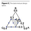
The slack, factorial design space of Figure 1 can be redrawn in terms of mixture coordinates as in Figure 5. The design space is twice as large as that of the desired design space. The grey area is the additional design space introduced by using the uncontrolled slack variable C in a slack, factorial design. Although the desired range for C was to be 0.3 to 0.4, because the maximum range of A and B each went to 0.4, C had to go to as low as 0.2. The formulations in the grey area may or may not work or be desired.The mixture design response equation was given in Equation 2. As already stated, the following equality holds:
A + B + C = 1 (3)
Equation 3 can be rearranged to give the following:
C = 1 – A – B (4)
If C in Equation 2 is substituted with Equation 4, a slack equation is obtained:
Property = aC + (aA – aC + aAC)A + (aB – aC + aBC)B + (aAB – aAC – aBC)AB – aACA2 – aBCB2 (5)
If we compare Equation 5 to Equation 1 we see the following:
b0 = aC (6a)
bA = (aA – aC + aAC) (6b)
bB = (aB – aC + aBC) (6c)
bAA = – aAC (6d)
bBB = – aBC (6e)
Equations 6a through 6e show that the effect of C on the Property is contained within the b0, bA, bB, bAA and bBB coefficients. This means that Equations 1 and 2 are equivalent. That is, a plot of the response surface of Equation 1 has been shown to be equivalent to that of Equation 2.
In the past, when an unsophisticated researcher viewed an analysis of variance table from a slack experimental design, if the variable A showed a significant effect, the researcher would attribute the effect to a change in A as manifested by the magnitude of the bA coefficient. But, looking at Equation 6b, if the bA coefficient is significant, the researcher doesn’t know if it is due to an effect from the variable A, the variable C or their interaction, AC. Similarly for the B variable, if the bB coefficient is significant, the researcher doesn’t know if it is due to an effect from the variable B, the variable C or their interaction, BC. However, the researcher can get an idea of the magnitude of the effects of C, AC and BC, by looking at the coefficients of b0, bAA and bBB. Then the researcher can do some mental gymnastics to determine how much C, AC and BC contribute to the effect of A or B. To my mind it is easier to use the mixture equation of Equation 2.
Closing Comments
The only time I would recommend using a slack, factorial design would be if it is absolutely known that C has no effect on the Property. That is, if the researcher knows ahead of time that aC, aAC and aBC are all zero.Another point for why I favor mixture designs is that even for the simple example of three ingredients, the quadratic mixture design has fewer experiments than the quadratic-slack, factorial design. However, if five ingredients are to be studied, for example, the quadratic mixture model requires only 15 experiments plus replicates and lack-of-fit points, while a quadratic-slack, factorial model requires 51 experiments.
Looking for a reprint of this article?
From high-res PDFs to custom plaques, order your copy today!


